
In recent years, we’ve witnessed a surge of new blockchains coming up, each with its unique set of features. More often than not, these chains are built atop something bigger, something more… open source – be it the Substrate based chains, the OP Stack, or the ZK Stack. This open-source foundation helps the general populace in utilizing the same technology these chains are built upon, to customize the functionality as one seems fit, and in turn benefit from the underlying security guarantees that come with Battle-Tested Open Source Code™.
Almost orthogonal to these development kits or technologies is something more generic… something fundamental that these environments astutely aspire towards. Something that is at the core of these chains, or rather these respective stacks, is that these chains always strive to be as efficient as possible. Ever since the advent of engineering, it feels as though we have been rushing to build the fastest and the most efficient piece of software possible – the true epitome of human excellence – encoded as 1s and 0s (citation needed). Those of us with backgrounds in Web 2.0 have already been exposed to a myriad of performance tuning and benchmarking disciplines that one would often fallback to, as required to do so by that eerie voice at 3 a.m. urging us even further:
“Psst… Hey! That insertion isn’t optimally amortized, you know”.
However, in our modern day Web 3.0 ecosystem, such functionally-complete tools and strategies are often lacking, or at least only recently nearing gradual maturity. So in the most generic sense of the word “emerging”, one would often find themselves receding to the daunting depths of static code reviews, in order to ascertain the eternal conjecture – doth thy code perform as one expecteth?
Performance Metrics
During the intense heat of subjective code reviews, one can often miss the nuanced realities of a bug, ever so graciously and subtly introduced amid the chaos of Monday mornings when the coffee machine breaks. In the way of all things Web 3.0, this can often lead to the ever so abominable security vulnerabilities, posing a significant threat to the stability of any blockchain, potentially bringing down any known chain to its distributed linked knees. Shudder.
The above scenario certainly begets the question – Is it possible to apply the sanctimonious performance optimization techniques, meticulously honed over years in the Web 2.0 domain, to the Web 3.0 space? Let’s examine the Substrate ecosystem as a case study. Substrate’s decision to run on today’s modern platform, i.e. the browser, and still perform exceedingly well, led to the adoption of WebAssembly (WASM). Consequently this choice quarantined off the majority of standard performance tuning strategies that one could employ in all things not WASM. However, in case of Substrate, the provision to benchmark any given code is exposed as a first-class citizen, which greatly improves the approach to decision-making regarding code and its performance, allowing for a nuanced application of optimization strategies within the Web 3.0 framework.
In the days of Web 2.0, the data-driven decisions usually materialized as CPU time or memory consumption metrics to objectively evaluate code performance. These were the critical metrics that one could rely on to answer concrete questions about code performance. In the blockchain space, different chains would almost certainly have different key performance metrics that ultimately govern the realms of what it means to run things efficiently. In case of Substrate, these critical metrics are designated to be the CPU time and the proof size, which appropriately encompass the weight (fee) of any given operation, encapsulating the essence of running processes efficiently in the blockchain environment.
Enter Benchmarks
The performance metrics of Substrate based chains are exposed via benchmarks, a concept well-known to the veterans of Web2. In the pursuit of optimizing code, high-quality benchmarks are employed to test and fine-tune specific segments, namely CPU time and/or memory consumption, providing a basis to categorize code implementations into distinct evaluations: “generally good”, “arguably acceptable”, or plain and simply “unambiguously unsatisfactory”. A methodological approach like this allows developers to make informed decisions about code optimizations that allows them to sleep soundly at night.
Substrate provides a user-friendly interface to accomplish this, especially when binaries are built under the runtime-benchmarks feature. This capability allows the underlying CLI to execute performance benchmarks. As the name implies, in most scenarios these are used to generate runtime weights – which is a Substrate way of saying how much fees need to be paid out for a specific operation. This, however, is not the only use case benchmarking can be applied to. For our work on Moonbeam, we often utilize this functionality when faced with challenges including, but not limited to:
- Making decisions on specific code-related trade-offs
- Optimizing and tuning our algorithms
- Making decisions on different kinds of data-structures we could employ
- Simply to understand our system under varying real-world scenarios
This comprehensive approach to benchmarking proves invaluable in enhancing our platform’s efficiency and reliability. Neat.
Making of a Benchmark
To effectively use benchmarks as decision making tools, it is essential to understand what goes into making a benchmark. While Substrate has great documentation on the underlying intricacies of writing a generic benchmark, it must be noted that such a benchmark must be written “correctly” in order to derive any meaningful conclusions from it. However, defining what“correct” means is often subjective and can vary heavily from case to case, or chain to chain. This variability underlines the importance of understanding the specific context and objectives of each benchmarking exercise to ensure its relevance and accuracy in informed decisions.
As a hypothetical example, say we are working on a staking feature in the codebase and wish to add a popular community requested feature:
Request: Delegations must be able to opt-in or opt-out into one of the following two categories:
- Those automatically compounding their rewards, and
- Those who don’t.
With a maximum of 100 delegation limit for each category.
After a good tech huddle, and multiple rounds of finely roasted coffee, it was promptly concluded that implementing such a feature could impact the critical path of the chain’s block production, and that a naive implementation might lead to significant performance degradation, at great inconvenience to users. Taking the above example, we can definitely start off with a rudimentary way to implement such a feature that looks just right, with the readily available code debt promise of:
“We’ll definitely optimize it later”.
Kaching.
After deciding to proceed, the next important step would be to write a benchmark for our naive implementation. The “correctness” of such a benchmark would come from white box knowledge of correctly accounting for the number of delegations to be paid out, the number of accounts that have opted-in for this feature, and those that have not.
So for our realistic benchmark, we assign the critical parameters that significantly govern the performance of our implementation. So far we’ve identified two:
- Number of delegations opting in
- Number of delegations opting out
We also ascertain realistic ranges that these values might take. In a real-world scenario with imposed constraints, we can either have no delegations to a maximum of 100, in each category. Sometimes it might be more complicated to establish these bounds, but identifying these critical parameters and their realistic bounds are an important piece of the equation for us to be able to derive meaningful conclusions in the end.
Substrate allows setting the parameters to a benchmark as follows:
let x in 0...10;
let y in 0...50;
The benchmark will thus run as a cross-product on the parameters x and y with dynamically generated increments based on the CLI (Command Line Interface) provided steps parameter. For our case we can write an example benchmark as follows:
payout_new_feature {
    let x in 0...100;  // number of delegations to payout that have opted-in
    let y in 0...100;  // number of delegations to payout that have opted-out

    for _ in 0..x {
        // setup delegations that have opted-in
    }

    for _ in 0..y {
        // setup delegations that have opted-out
    }
}: {
    // benchmark the unit
    <Pallet<T>>::pay_rewards();
} verify {
    // assert all rewards were paid out
}
In order to run this benchmark, we compile the binary in release mode so our benchmarks are as realistic as possible, along with the runtime-benchmarks flag:
cargo build --release --features runtime-benchmarks

# generates "./target/release/my_binary"
The generated binary can then be used to execute the benchmark we just created as follows:
my_binary benchmark pallet \
    --pallet pallet_example \
    --extrinsic payout_new_feature \
    --steps 50 \
    --repeat 3 \
    --json-file raw.json
The –pallet parameter is quite ubiquitous to substrate developers and basically defines where the functionality resides, with –extrinsic specifying the benchmark’s name. The –steps parameter can be used to fine tune the interpolation within the bounds of the parameters – effectively using a higher step count increases the quality of the benchmark at the cost of execution time. We –repeat the benchmark finite number of times to smoothen out any spikes. And finally, the –json-file which will contain our benchmarked metrics.
Upon executing the above command, we get the json file as output containing the following data:
[
  {
    "pallet": "pallet_example",
    "instance": "Example",
    "benchmark": "payout_new_feature",
    "db_results": [
      {
        "components": [
          ["x", 50],
          ["y", 100],
        ],
        "extrinsic_time": 8727,
        "storage_root_time": 20860,
        "reads": 50,
        "repeat_reads": 100,
        "writes": 20,
        "repeat_writes": 0,
        "proof_size": 35699
      },
      // other entries with variations of `x` and `y` ...
    ]
    // ...
  }
]
This generated file is already of great use to us since for smaller datasets we can simply glance over the values to determine the general performance of the rudimentary code that was just written.
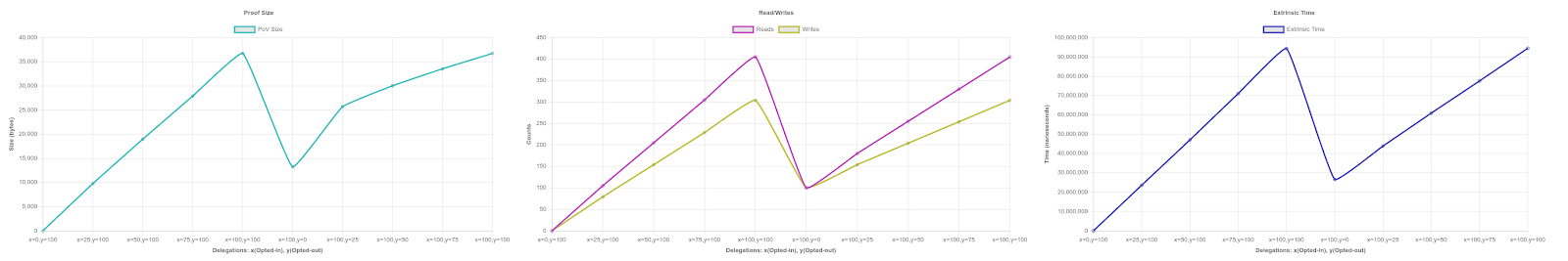
The line charts above help us understand how our code is behaving when a certain number of delegations have either opted-in or opted-out during the payout. Noting the proof size we can also estimate if a produced block during the scenario might be considered “too heavy”.
To take matters further, we can even easily chart this data as a heatmap, with the x and y parameters on their respective axis and the values for either proof_size or extrinsic_time with the heat color, using any tool of choice.
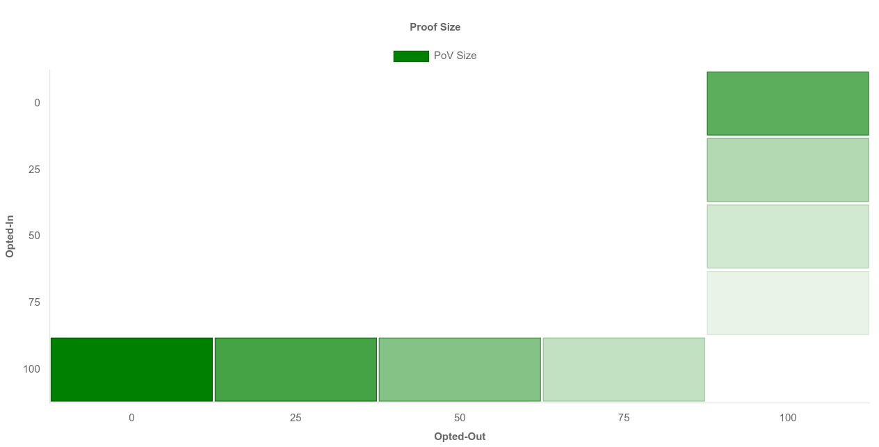
Such visualizations are particularly useful when answering questions like, “How would my network look like if I have both sets either – fully filled, partially empty, or fully empty?”. These visualizations would almost always provide the required information of how the network would behave in these varied situations identified earlier.
Visualizing Multi-Dimensions
It’s good that we have access to all variations of the x and y and their respective performance metrics, but sometimes it might be hard to visualize n-parameters on screen (where n > 2), and here’s where things get interesting. Substrate allows us to override the parameters via command line that can be used to get the associated metrics for a variety of custom scenarios. For example, we can define 5 scenarios of interest in our example:
- Both sets fully empty (0, 0)
- Both sets fully filled (100, 100)
- Both sets partially filled (50, 50)
- Everyone opted-in, but other set is empty (100, 0)
- Everyone opted-out, but other set is empty (0, 100)
These scenarios are majorly identified on a case by case basis and are highly subjective to a specific benchmark, or the code under review.
To benchmarks against these custom scenarios, we can execute the following commands:
my_binary benchmark pallet
	--pallet pallet_example \
	--extrinsic payout_new_feature \
	--steps 1 \
	--repeat 3 \
	--json-file raw_empty.json \
	--low "0,0" \
	--high "0,0"
my_binary benchmark pallet \
	--pallet pallet_example \
	--extrinsic payout_new_feature \
	--steps 1 \
	--repeat 3 \
	--json-file raw_full.json \
	--low "100,100" \
	--high "100,100"
my_binary benchmark pallet \
	--pallet pallet_example \
	--extrinsic payout_new_feature \
	--steps 1 \
	--repeat 3 \
	--json-file raw_partial.json \
	--low "50,50" \
	--high "50,50"
my_binary benchmark pallet \
	--pallet pallet_example \
	--extrinsic payout_new_feature \
	--steps 1 \
	--repeat 3 \
	--json-file raw_all_opted_in.json \
	--low "100,0" \
	--high "100,0"
my_binary benchmark pallet \
	--pallet pallet_example \
	--extrinsic payout_new_feature \
	--steps 1 \
	--repeat 3 \
	--json-file raw_all_opted_out.json \
	--low "0,100" \
	--high "0,100"
The above commands basically set the lower and upper bounds for x,y to fixed values in each execution as we desire to obtain a singular entry in the json file which contains the performance metrics of interest. These json files containing singular values can then easily be aggregated by an appropriate tool of choice to generate discrete points on the all too familiar x-y axis, with the y-axis being the value of either proof_size, the extrinsic_time, reads, etc. and the x-axis is simply the discrete scenarios we have.
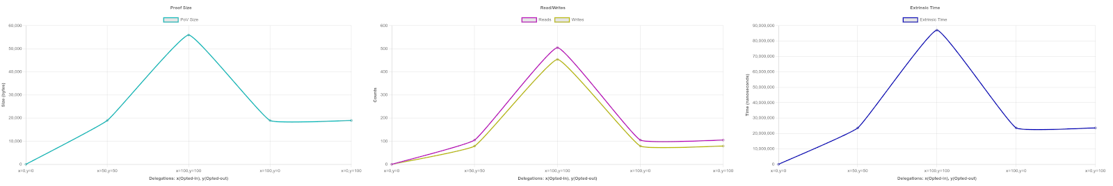
Visualizing this data can often give us a better understanding of trends as they may arise, and are especially important when performance tuning for specific use-cases. In the case above we see that our naive implementation increases in a non-linear fashion at higher values of x and y, with the last two scenarios of (100,0) and (0,100) being comparable to (50,50). We can thus also state that our implementation is neither biased towards the delegations that have opted-in nor to the ones that have opted-out.
Comparing Implementations
To go one step further, this same approach is quite useful to evaluate different algorithms or even storage choices, especially in blockchains where storage is a critical resource. The competing implementations can be compiled as competing binaries – my_binary1, my_binary2, my_binary3 and be subjected to the same benchmark defined in each.
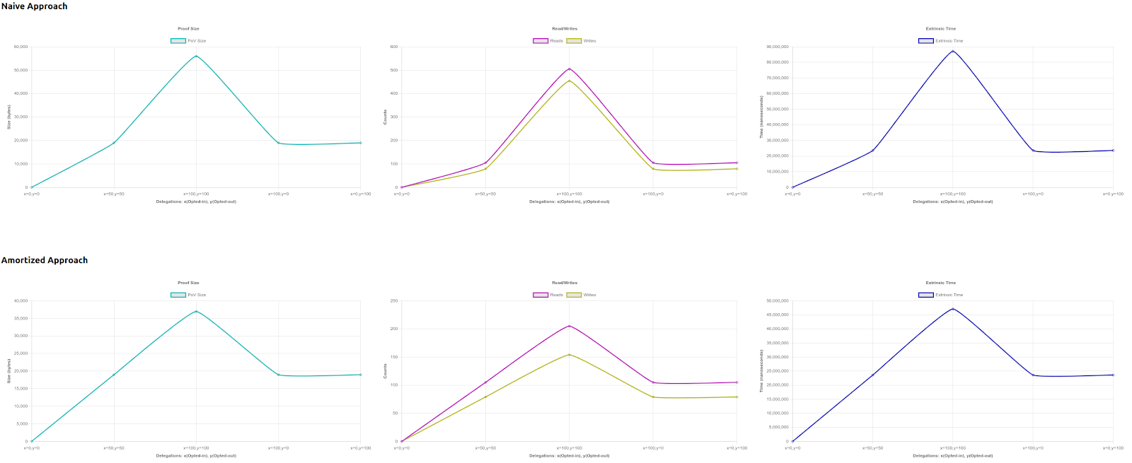
In the example above, where the first approach is compared against a new implementation, we can clearly identify that our implementation is now linear with respect to the number of delegations that have either opted-in or opted-out, effectively performing better at higher network load.
Final Thoughts
Leveraging the approaches mentioned above and generating the JSON data points, we can understand our own code, predict its behavior in different real-world network scenarios, and evaluate the implicit tradeoffs of our different approaches better. Perhaps good enough to not warrant that extra cup of coffee that late in the night. And perhaps, just perhaps, help us adequately answer that voice at 3 a.m. – Is that insertion really NOT appropriately amortized?.